O C E A N M A P P I N G
Topics, methods and subjects learned:
- working with WOD 2009 data
- Ocean Data Viewer
- working with large datasets
- data table editing and configuration
- querying relevant data
- summarizing data
- adding X,Y data to create point shape files
- inverse weighted grids
- map algebra
- working with ArcGIS shaded relief layers
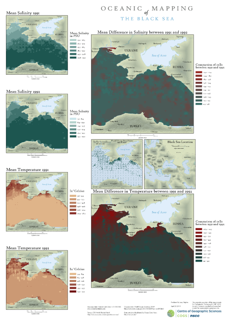
Temperature and Salinity 1991-1992
Created in Notepad, Microsoft Excel and ArcMap 9.3.1.
Initially, data was selected by geographic location from the World Ocean Database 2009's website. This data was available in a .gz format that was read by Ocean Data Viewer. The points were shown in their geographic global context and displayed the data that points carried when clicked. The data was then exported out of ODV as a table. This table had to be heavily edited to remove rogue values, missing values, and null values. Once all was in order and the proper headings were established, the table was brought into an ArcMap session. Here, the desired values were queried to provide the points necessary for grid creation. These queries were exported and then summarized by average. The resulting shape file was given a modified Mercator projection.
Under Spatial Analyst Interpolate - Raster function - the inverse distance weighted option was selected to create the grids used. A cell size of 1000 was used for all. Once two grids had been generated the following command was issued with Raster Calculator in order to obtain the difference between them:
Diff = Salinity1992 - Salinity1991
The resulting grids were symbolized by class and given appropriate colour schemes.
